Two Way ANOVA Calculator
Factorial ANOVA - Balanced design
Fixed effects, Mixed effects, Random effects and Mixed repeated measures
Unbalanced two way ANOVAReplications are observations of the same combination of factors A and B.
Balanced two factor ANOVA with replication - enter all the replications in one cell separated by Enter or , (comma).
ANOVA without replication - enter one value per cell.
The tool ignores empty cells or non-numeric cells.
Balanced two factor ANOVA with replication - enter all the replications in one cell separated by Enter or , (comma).
ANOVA without replication - enter one value per cell.
The tool ignores empty cells or non-numeric cells.

Information
Models
There are many possible models, this calculator deal currently only with the following balanced models:- Fixed effect model (A-Fixed, B-Fixed), no repeats - both factors are fixed.
- Mixed effect model (A-Random, B-Fixed), no repeats - factor A is random, factor B is fixed, each subject is measured only once.
- Mixed effect model (A-Fixed, B-Random), no repeats - factor A is fixed, factor B is random, each subject is measured only once.
- Random effect model (A-Random, B-Random), no repeats
- Mixed repeated measures (A-Fixed, B-Repeated) - factor A is fixed, factor B uses the same subject for all the categories.
What is balanced model?
The balanced design has the same number of observations in each cell - each combination of factor.Currently this calculator supports only the balanced design.
When the model is unbalanced, it causes correlation between the factors and the interaction if it is proportional, and also between the factors if it is unbalance but not proportional.
hence you don't know how to divide the shared sum of squares between the two factors.
There are several methods how to deal with the shared sum of squares.
Type I - sequenceial, the first some of squares (SS) you calculate get the shared some of squares, in this case the order is matter!
Type II - conservative, it assumes there is no interaction between the factors, it ignores the shared SS between the factors. Type III - it assumes there is interaction between the factors, it ignores all the shared SS between the factors and between the factors and the intercation.
Targets
The two way ANOVA test checks the following targets using sample data.- Checks if the difference between Factor A averages of two or more categories is significant
- Checks if the difference between Factor B averages of two or more categories is significant
- Checks if there is an interaction between Factor A and Factor B
The F statistic represents the ratio of the variance between the groups and the variance inside the groups. Unlike many other statistic tests, the smaller the F statistic the more likely the averages are equal.
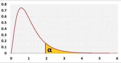
Right-tailed F test, for ANOVA test you can use only the right tail. Why?
b - the number of categories in variable B, number of columns.
ni - sample side of category i of variable A (row i).
nj - sample side of category j of variable B (column j).
ni,j - sample side of cell i,j (row i, column j). In the balance ni,j=n/(a*b)
n - overall sample side, includes all the groups (Σni,j, i=1 to a, j=1 to b).
Ȳi - average of all the observations of category i of variable A (row i).
Ȳj - average of all the observations of category j of variable B (column j).
Ȳ - overall average (ΣYi,j,k / n, i=1 to a, j=1 to b, k=1 to ni,j).
sub - number of subjects per cell, cell is one combination of variable A and variable B. For the balance design: N=a*b*sub.
Ȳi,s - subject's average, ΣYi,j,s for subject i,s ,the average of all the observations of subject s of category j of variable B (column j).
Ȳ - overall average (ΣYi,j,s / n
SSA - the squared differences related to the effect of variable A. You compare the average of every category to the total average. The same value as the sum of squares between groups in one way ANOVA.
SSB - the same as SSA, for variable B.
SSAB - the squared differences related to the effect of the combination of variable A and variable B in each cell, Since we try to understand the influence of the interaction AB, the interaction of the specific value of variable A and the specific value of variable B, we take the average of each cell, remove the influence of variable A and variable B, and compare to the total average.
A effect = Ȳi - Ȳ
B effect = Ȳj - Ȳ
AB effect = Cell average - A effect - B effect - Total average.
= Ȳi,j - (Ȳi - Ȳ) - (Ȳj - Ȳ) - Ȳ.
= Ȳi,j - Ȳi - Ȳj + Ȳ.
Take the square of each difference
Ȳi,j - Ȳi - Ȳj + Ȳ)2.
Count the square differences of each value in the cell, hence multiply by the sample size of each cell (ni,j).
SSAB=ΣiaΣjbni,j(Ȳi,j - Ȳi - Ȳj + Ȳ)2
A sample from the entire groups' population.
There is no pattern about the difference between the schools, and if there will be a pattern, it will be another factor, like school's size.
Each school is not important by itself.
A effect: Ȳi - Ȳ.
B effect: Ȳj - Ȳ.
Two-way ANOVA
Hypotheses
H0: Interaction(AiBj) = 0 (∀ i = 1 to a, j = 1 to b)
There is no interaction between variable A and variable B, i.e., for all the cells, the effect of variable A on the cells' means is not depend on the effect of variable B, and vice versa.
Factor A: H0: μ1 = .. = μa
There is no difference in the means of variable A categories.Factor B: H0: μ1 = .. = μb
There is no difference in the means of variable B categories.H0: Interaction(AiBj) = 0 (∀ i = 1 to a, j = 1 to b)
There is no interaction between variable A and variable B, i.e., for all the cells, the effect of variable A on the cells' means is not depend on the effect of variable B, and vice versa.
Two-way ANOVA tests formulas
| Fixed Model | Mixed Model | Random Model | Mixed Repeated | ||||
| FA= | MSA | FA= | MSA | FA= | MSA | FA= | MSA |
| MSE | MSAB | MSAB | MSSWA | ||||
| FB= | MSB | FB= | MSB | FB= | MSB | FB= | MSB |
| MSE | MSE | MSAB | MSBSWA | ||||
| FAB= | MSAB | FAB= | MSAB | FAB= | MSAB | FAB= | MSAB |
| MSE | MSE | MSE | MSBSWA | ||||
F distribution
Assumptions
- The dependent variable is continuous (ratio or interval)
- Two categorical independent variables
- Independent observations (no repeated measure)
- The residuals distribution is normal
- Homogeneity of variances, a similar variance for each cell
Required Sample Data
| Sample data from all compared groups |
Parameters
a - the number of categories in variable A, number of rows.b - the number of categories in variable B, number of columns.
ni - sample side of category i of variable A (row i).
nj - sample side of category j of variable B (column j).
ni,j - sample side of cell i,j (row i, column j). In the balance ni,j=n/(a*b)
n - overall sample side, includes all the groups (Σni,j, i=1 to a, j=1 to b).
Ȳi - average of all the observations of category i of variable A (row i).
Ȳj - average of all the observations of category j of variable B (column j).
Ȳ - overall average (ΣYi,j,k / n, i=1 to a, j=1 to b, k=1 to ni,j).
Repeated measures ANOVA
s - represent the order of subject in category i (subject 1 in category 1 is different than subject 1 in category 2)sub - number of subjects per cell, cell is one combination of variable A and variable B. For the balance design: N=a*b*sub.
Ȳi,s - subject's average, ΣYi,j,s for subject i,s ,the average of all the observations of subject s of category j of variable B (column j).
Ȳ - overall average (ΣYi,j,s / n
Results calculations
Sum of squares
The sum of squares accumulates the squared differences related to the effect we try to estimate.SSA - the squared differences related to the effect of variable A. You compare the average of every category to the total average. The same value as the sum of squares between groups in one way ANOVA.
SSB - the same as SSA, for variable B.
SSAB - the squared differences related to the effect of the combination of variable A and variable B in each cell, Since we try to understand the influence of the interaction AB, the interaction of the specific value of variable A and the specific value of variable B, we take the average of each cell, remove the influence of variable A and variable B, and compare to the total average.
A effect = Ȳi - Ȳ
B effect = Ȳj - Ȳ
AB effect = Cell average - A effect - B effect - Total average.
= Ȳi,j - (Ȳi - Ȳ) - (Ȳj - Ȳ) - Ȳ.
= Ȳi,j - Ȳi - Ȳj + Ȳ.
Take the square of each difference
Ȳi,j - Ȳi - Ȳj + Ȳ)2.
Count the square differences of each value in the cell, hence multiply by the sample size of each cell (ni,j).
SSAB=ΣiaΣjbni,j(Ȳi,j - Ȳi - Ȳj + Ȳ)2
Fixed and Random Effects
The fixed and random effects are related to the independent variables ().Fixed Effect
The effect is constant across individuals.- The categories of the variable contains the entire categories' list
- The effect of this variable is interesting. The difference between the categories is important
- There is no know pattern on the difference between the categories
Random Effect
The effect vary across individuals, the individuals may be people, products.- The categories' list is only a sample from the entire categories' list
- The effect of this variable is not interesting by itself. The difference between the categories is not important.
- There is no know pattern on the difference between the categories
A sample from the entire groups' population.
There is no pattern about the difference between the schools, and if there will be a pattern, it will be another factor, like school's size.
Each school is not important by itself.
When you change the interaction field or the model, the following ANOVA table and diagram will be adjusted!
ANOVA table - with interaction
| Source | Degrees of Freedom (DF) | Sum of Squares (SS) | Mean Square (MS) | F statistic | p-value |
|---|---|---|---|---|---|
| Factor A (rows) Between the categories of factor A | DFA = a - 1 | SSA = Σiani(Ȳi-Ȳ)2 | MSA = SSA / DFA | FA = MSA / MSE | P(x > FA) |
| Factor B (Columns) Between the categories of factor B | DFB = b - 1 | SSB = Σjbnj(Ȳj-Ȳ)2 | MSB = SSB / DFB | FB = MSB / MSE | P(x > FB) |
| Interaction AB Between the cells after reducing factor A and factor B effects | DFAB = (a - 1)(b - 1) | SSAB=ΣiaΣjbni,j(Ȳi,j - Ȳi - Ȳj + Ȳ)2 | MSAB = SSAB / DFAB | FAB = MSAB / MSE | P(x > FAB) |
| Error Within the cells | DFE = n - a*b | SSE=ΣiaΣjbΣkni,j(Yi,j,k - Ȳi,j)2 | MSE = SSE / DFE | ||
| Total All the deviations from the average | DFT = n - 1 | SST=ΣiaΣjbΣkni,j(Yi,j,k - Ȳ)2 SST=Sample Variance*(n-1) SST=SSA+SSB+SSAB+SSE | MSE = S2 = SST / (n - 1) |
Sum of squares diagram - with interaction
In the following diagram you may see the differences per each observation Yi,j,k that used to calculate the sum of squares.A effect: Ȳi - Ȳ.
B effect: Ȳj - Ȳ.
Interaction effect (AB): Yi,j - Ȳi - Ȳj + Ȳ.
Error: Yi,j,k - Ȳi,j.
Total effect: Yi,j,k - Ȳ.Error: Yi,j,k - Ȳi,j.