One Way MANOVA Calculator
MANOVA calculator with calculation steps, Wilks' Lambda, Pillai's Trace, Hotelling-Lawley Trace, Roy's Maximum Root.
It is followed by a Univariate ANOVA or multiple comparisons MANOVA, Box’s M test, Mahalanobis Distance test, and SW test.
The tool ignores empty cells or non-numeric cells.

MANOVA online
One-way MANOVA determines whether there is a significant difference between the averages of two or more independent groups.
An analysis of variance (ANOVA) is a special case of a multivariate analysis of variance (MANOVA)
As opposed to one-way ANOVA, where one dependent variable (Y) is assigned to each subject, MANOVA has several dependent variables (Y1, Y2, ..., Yp). Using the MANOVA test provided more power than running a one-way ANOVAs test for each dependent variable. The ANOVA examines only variances, while the MANOVA examines the variances, but also correlations. Correlations between dependent variables provide more information and therefore increase the test power.
When using several ANOVA tests you need to correct the significance level (α), to avoid a large type I error, but in MANOVA there is no need to correct the significance level.
Targets
The one-way MANOVA test compares the average of one or more dependent variables (Yi) across two or more groups when every subject contains a value for each dependent variable. Practically for one dependent variable we use the ANOVA.
When performing the one-way MANOVA test, we try to determine if the difference between the vector averages reflects a real difference between the groups, or is due to the random noise inside each group.The F statistic represents a connection of the SSCP between the groups (H) and the SSCP within the groups (E) error. Unlike many other statistic tests, the smaller the F statistic the more likely the averages are equal.
| F = | V | * | df₂ |
| s - V | df₁ |
MANOVA test statistics
As with ANOVA, we compare between-groups to within-groups using the F distribution, but instead of using only the Sum of Squares (variances), we use both Sum of Squares and Cross Products (variances and covariances of dependent variables).
A similar result can be obtained by one of the following statistics: Wilks' Lambda, Pillai’s trace, Hotelling-Lawley trace, Roy’s maximum root.
Each statistic examines the variance in data in a different way depending on how it combines the dependent variables
In general, Wilks' lambda is the most commonly used statistic due to its simplicity, but we recommend to use the Pillai's trace. The Pillai's trace offers the greatest protection against Type I errors, it is a bit more powerful and more more robust against violations of the homogeneity assumption for covariance matrices.
Parameters
p - number of dependent variables [Y1, Y1, ... , Yp], number of columns.g - number of groups/treatments, number of rows.
n - number of subjects, number of observations for one dependent variable (Yi), the number of values in one column.
λi - eigen value i.
Wilks' Lambda
| Λ = | |E| |
| |H + E| |
| Λ = π | 1 |
| 1 + λi |
Wilks' Lambda formula
| F = | 1 - Λ1/b | * | df₂ |
| Λ1/b | df₁ |
| a = n - g - | p - g + 2 |
| 2 |
| b = | p²(g - 1)² - 4 |
| p² + (g - 1)² - 5 |
| c = | p(g - 1) - 2 |
| 2 |
df₂ = a*b - c
Pillai’s trace
V = tr(H(H + E)-1), tr is the trace of the matrix| V = Σ | λi |
| 1 + λi |
Pillai’s trace formula
| F = | V | * | df₂ |
| s - V | df₁ |
v = n - g.
| u = | p(g -1) - 2 |
| 4 |
df₁ = s*(2m + s +1)
df₂ = s*(2u + s +1)
Hotelling-Lawley trace
U = tr(HE-1)| U = Σ( | 1 | ) |
| 1 + λi |
Hotelling-Lawley Trace formula
| F = | U | * | df₂ |
| s | df₁ |
df₂ = s*(s*u + 1)
Roy’s maximum root
Θ = Max(λi)Roy’s maximum root formula
| F = Θ | df₂ |
| df₁ |
df₂ = n - r - 1
MANOVA test power
We use the noncentral F distribution for the alternative assumption (h1). The non central parameter is: Wilks' Lambda:
ncp = f2*n*b
Pillai’s trace and Hotelling-Lawley trace:
ncp = f2*n*s
Currently for Roy's maximum root statistic we calculate the power of Pillai’s trace.
How to use the MANOVA calculator?
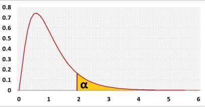
- Significance level (α): A p-value less than the significance level is statistically significant.
Researchers usually use 0.05, but if the price of a mistake is big, they may use a smaller value like 0.01. - Advanced fields - for sample size
WE use this fields to calculate the priori test power. When planning the experiment, you should choose the effect size that the test should identify. You should choose the sample size before conducting the research. We added this field to alert users that didn't calculate the sample size or did it incorrectly.
If you use the calculator for homework you may ignore these fields.
Effect - If you don't know the required effect size, you may use the 'effect' field. The default is 'Medium', if you change the value, it will change 'effect type' to 'Standardized effect size' and fill the proper value per Cohen's suggestion in the 'effect size' field. (0.2: Small, 0.5: medium, 0.8: large) The calculator will not use this field when pressing the 'calculate' button.
Effect type
f - effect size.
f2 - effect size.
ηp2 - partial ETA squared
Effect size - the value that you want the test to be able to identify. You need a larger sample size to be able to identify a smaller effect size.ηp2 = df₁*F df₁*F + df₂ - Rounding - how to round the results?
When a resulting value is larger than one, the tool rounds it, but when a resulting value is less than one the tool displays the significant figures. - How to enter data?
Enter data in a table - several subjects in each cell, separated by 'enter' comma or space.
Along the row, the order of the subjects is the same.
Enter data from excel - the data should contain 3 columns: Group, Y, Value. One row represents one DV of one subject.
If the data contains the subject column, don't copy this column.
Copy the raw data with the top header, and paste it into the calculator. You may copy from Excel, 'Google sheets', or any tool that separates data with tab and line feed. Copy the entire block, and include the header. - Step-by-step - switch on to get the calculation steps.
Assumptions
- Independent - each observation is randomly selected.
- Continuous dependent variables (ratio or interval)
- Linearity between all the dependent variables
- Multivariate normality - for all the dependent variables, MANOVA is robust against departures from multivariate normality
- One categorical independent variable, groups or treatments
- Each subject contains data for all the dependent variables
- Homogeneity of variance and covariance - equality of covariances matrices for all groups
Multivariate Outlier - Mahalanobis Distance
Calculate for each subject:
Ȳ - average vector, contain the averages of each column.
Yi-Ȳ: one row in the DTotal matrix.
df = p. (number of dependent variables)
When p-value < 2*α : Suspected Outliers.
Required Sample Data
Sample data from all compared groups
Results calculations
Following the calculation formulas with example.1. Averages
Calculate average of each cell, and each column (Yi). To calculate the average of a column use the data in all the cells in this column.2. SSCP groups
Calculate the Square and Cross Products matrix (SSCP) for each group.1. Calculate the differences matrix (D), by subtracting the relevant group's average from each observation.
2. Calculate the Sum of Square and Cross Products matrix (SSCP) using the following matrix form formula:
3. Within-groups SSCP (SSCPW)
Add up the SSCP matrices for all the gropus:4. SSCP total
Similarly to the SSCP groups calculation but in this case use the entire columns.Calculate the Square and Cross Products matrix (SSCP) for the all the groups togather.
1. Calculate the differences matrix (D), by subtracting the total's average from each observation.
2. Calculate the Sum of Square and Cross Products matrix (SSCP) using the following matrix form formula: