Z-test vs t-test
When to use the z-test vs t-test?
When you know the population standard deviation you should use the z-test, when you estimate the sample standard deviation you should use the t-test.The t-distribution has heavier tails (Leptokurtic Kurtosis) than the normal distribution to compensate for the higher uncertainty because we estimate the standard deviation. (the standard deviation of the standard deviation statistic)
Usually, we don't have the population standard deviation, so we use the t-test.
When the sample size is larger than 30, should I use the z-test?
You should use the t-test!The t-test is always the correct test when you estimate the sample standard deviation. I guess the reason for the confusion is historical. The degrees of freedom equal sample size minus one. When the sample size is greater than 30, the t-distribution is very similar to the normal distribution.
The t-distribution limit at infinity degrees of freedom is the normal distribution.
In the past, people used tables to calculate the cumulative probability. For the t-table you need to have a separate set of data for any DF value, hence the Z-Table is more detailed and more accurate than the t-table.
Z distribution vs t distribution
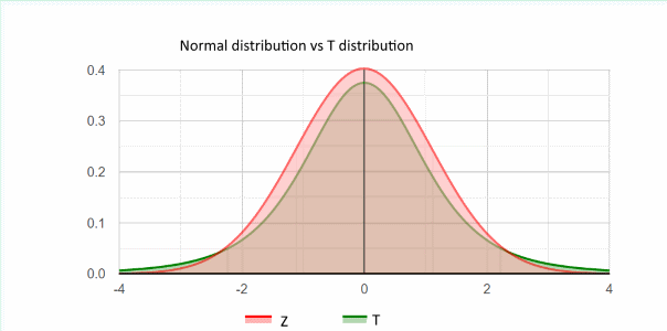
You may see the Leptokurtic kurtosis shape of the t-distribution (DF=4), compares to the Normal distribution (Z).
As with any distribution, the area of both distributions equals one. The normal distribution is higher close to the center, while the t-distribution is higher on the tails.
Z-test type I error - using sample standard deviation
The following simulation ran over 300,000 samples of a normal population and compares the sample mean to the true mean, using the t-test and the z-test with a significance level of 0.05.
In both tests, we use the sample standard deviation.
Since the null assumption is correct, we expect the type I error, the probability to reject the correct H0, to be 0.05. (as this is the significance level definition). For the z-test, even for a sample size of 30, the type I error is ~0.06 instead of 0.05, this means that in the simulation we rejected 0.06 of the cases, instead of 0.05!
For the t-test, the type I error is around 0.05, as expected.
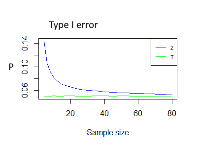
The following charts show the actual type I error in the simulation
Blue Z - The actual type I error for the z-test when using the sample standard deviation.
Green T - The actual type I error for the t-test.
T vs Z - type I error chart
Z-test Type I error table
Following the simulation results of type I error, when using sample standard deviation in z-test.
| Sample Size | Type I error |
| 4 | 0.1443 |
| 5 | 0.1214 |
| 6 | 0.1069 |
| 7 | 0.0973 |
| 8 | 0.0903 |
| 10 | 0.082 |
| 12 | 0.0758 |
| 15 | 0.0697 |
| 17 | 0.068 |
| 20 | 0.0652 |
| 25 | 0.0615 |
| 30 | 0.0595 |
| 35 | 0.0589 |
| 40 | 0.0573 |
| 45 | 0.0563 |
| 50 | 0.0558 |
| 60 | 0.0546 |
| 80 | 0.0523 |
Z-test type I error - using population standard deviation
The following simulation ran over 300,000 samples of a normal population and compared the sample mean. This time we know the population standard deviation.
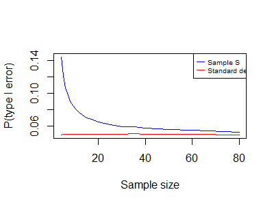
Blue Z (S) - The actual type I error for the z-test when using the sample standard deviation.
Red Z (σ) - The actual type I error for the z-test when using the population standard deviation.
We should use the more accurate population standard deviation, and not the estimated sample standard deviation, and the next simulation chart is as expected.
Why the following chart looks the same as the t-test vs z-test - type I error chart?
The green line, in the previous chart, shows the type I error for the t-test when using the correct test (sample S).
The red line, in the current chart, shows the type I error for the z-test when using the correct test (σ).
We expect that For any statistical test, the type I error will be around the significance level (α0).
Z-test type I error chart
Simulation - R code
t-test vs z-test
library(BSDA)
reps < - 300000 # number of simulations
n1 < - 100; # sample size
#population
sigma1 < - 12# true SD
mu1 < - 40# true mean
n_vec < -c(4,5,6,7,8,10,12,15,17,20,25,30,35,40,45,50,60,80)
pvt < - numeric (length(n_vec))
pvz < - numeric(length(n_vec))
j=1
for (n1 in n_vec) # sample size
{
pvalues_t < - numeric(reps)
pvalues_z < - numeric(reps)
set.seed(1)
for (i in 1:reps) {
x1 < - rnorm(n1, mu1, sigma1) #take a smaple
s1=sd(x1)
pvalues_t[i] < - t.test(x1,x2=NULL,mu = mu1,alternative="two.sided")$p.value
pvalues_z[i] < - z.test(x1, y=NULL, alternative = "two.sided", mu = mu1, sigma.x = s1)$p.value
pvalues_z[i] < - z.test(x1, y=NULL, alternative = "two.sided", mu = mu1, sigma.x = sigma1)$p.value
}
pvt[j] < - mean(pvalues_t < 0.05)
pvz[j] < - mean(pvalues_z < 0.05)
j=j+1
}
Z-test with sample S vs z-test with σ
We used the same code, but instead of t-test we used z-test with sigma1:
pvalues_z0[i] < - z.test(x1, y=NULL, alternative = "two.sided", mu = mu1, sigma.x = sigma1)$p.value