Propensity Score Matching Generator

When to use the PSM?

You may use the propensity score analysis when you couldn't randomized the treatment. The propensity score matching help to reduce the effect of the confounding variables (covariates) by matching similar subjects between treatment group and the control group.

What is propensity score

Most often, propensity scores are estimated as the likelihood that a person would be assigned or self-select into a treatment condition. [1].
For example, the propensity score can be estimated using a logistic regression model.

Balance Estimation

1. Covariate.
2. Treatment mean - the average value of the covariate in the treatment groups.
3. Control mean - the average value of the covariate in the control groups.
4. Std Bias (SB) - standardized bias, the standardized mean difference.

Compares the distribution of each covariate between the treatment group and the control group.
A balanced propensity score does not imply balanced covariates (Austin, 2009), and vice versa.
For example, when using logistic regression to calculate the score, the score represents the probability of treatment based on the covariates.
Different combinations of covariates may lead to similar treatment probabilities (scores).
Since the data is matched using the score, it may result in non-balanced matching.

Standardized Mean Difference

There is no clear standard for the S_B value of a balanced covariate. However, |S_B| should be smaller than 0.2, or preferably smaller than 0.1 for important covariates.

Numerical Covariates

Calculates the standardized difference between the estimated mean of the treatment group and the estimated mean of the control group.

Categorical Covariates

For each value of the categorical covariate, calculates the standardized difference between the estimated proportion of the treatment group and the estimated proportion of the control group.

Variance ratios balance

The variance ratio is the ratio of the variance of a covariate in the treatment group to the variance of the same covariate in the control group.
For a well-balanced matching, we expect these variances to be similar, with the ratio close to 1.
The variance ratio should fall between 0.5 and 2 (Rubin, 2001).

Input Data Structure

1. ID - The first column contains the unique ID. The input data must include the ID column for data completeness, but the PSM process will not use it.
2. Covariates - The subsequent columns represent covariates, which can be either numerical or categorical variables. These covariates are independent variables that are not of primary interest.
3. Treatment - The second-to-last column represents the treatment. This is the key independent variable, and it should contain only values of 1 or 0 (1 indicates treatment, 0 indicates no treatment).
4. Output - The last column contains numerical data, representing the dependent variable.

How to use the PSM calculator

PSM calculator with optional Excel file input. Propensity score estimation is performed using logistic regression, and matching is done using the nearest neighbor method, with an optional caliper.

How to enter data?

• Enter raw data directly - usually you have the raw data.
  a. Enter the name of the group.
  b. Enter the raw data separated by 'comma', 'space', or 'enter'. (*you may copy only the data from excel).
• Enter raw data from excel

  Enter the header on the first row.

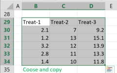
  1. Copy Paste
     
     • a. copy the raw data with the header from Excel or Google sheets, or any tool that separates data with tab and line feed. copy the entire block, include the header .
     • Paste the data in the input field.
  2. Import data from an Excel or CSV file.
     When you select an Excel file, the calculator will automatically load the first sheet and display it in the input field. You can choose either an Excel file (.xlsx or .xls) or a CSV file (.csv).
     To upload your file, use one of the following methods:
     1. Browse and select – Click the 'Browse' button and choose the file from your computer.
     2. Drag and drop – Drag your file and drop it into the 'Drop your .xlsx, .xls, or .csv file here!' area.
     Once the file is uploaded, the PSM calculator will display the data from the first sheet in the input field.
     Now, the 'Select sheet' dropdown will be populated with the names of your sheets, and you can choose any sheet.
  3. Filter Data
     When using the 'Enter data from Excel' option, you can filter the data by clicking the following icon above the header:
     You may select one or more values from the dropdown. Please note that the filter will include any value that contains the values you choose.

Assumptions

1. The treated subjects and the control subjects have a similar probability of receiving the treatment.
2. All subjects receive the same type and amount of treatment.
3. No general equilibrium effect - the control subjects don't get the treatment indirectly.
4. Sufficient overlap between the treated group and the control group.
5. Conditional independent - the outcomes (y) are independent of the treatment.
6. No Hidden Bias: All confounding variables are included in the model

Logistic regression parameters

1. Score Calculation:
   Logistic Regression - the columns Name-1, Name-2, etc. are covariates used to calculate the score using logistic regression.
   Existing score column - in this case, there is only one column, Name-1, which represents the score.
2. Learning Rate(α): The learning rate represents the size of the gradient step in each iteration. It controls how much the coefficients are adjusted during each iteration of the optimization process. A smaller alpha means smaller steps in gradient descent, which can lead to more precise convergence but might require more iterations and longer calculation time.
   Common alpha values typically range from 0.1 to 0.001 when using a constant learning rate (decay rate = 1).
   When using a decayed learning rate (decay rate < 1), you may start with a higher learning rate, typically ranging from 1 to 10.
3. Decay Rate:
   The decay rate refers to the reduction of the learning rate over time. A large learning rate allows faster training, while a small learning rate offers more accuracy by reducing the chance of overshooting the optimal point. Gradually decreasing the learning rate can combine the benefits of both approaches — it starts fast and becomes more accurate as it slows down toward the end of the optimization process. In each iteration:
   In any iteration in which the cost does not decrease, the algorithm reduces the learning rate as follows:
   Learning Rate = Learning Rate * Decay Rate.
4. Replacement:
   With replacement – when matching, the same control subject may be matched more than once (for ATT), or the same treated subject may be matched more than once (for ATC).
   Without replacement – each subject is matched only once.
   
5. Effect Type (Estimand):
   On Treated (ATT) – Average Treatment Effect on the Treated; for each treated subject, match the best control subject.
   On Controls (ATC) – Average Treatment Effect on the Controls; for each control subject, match the best treated subject.
   
6. Penalty(λ): This parameter controls the amount of regularization applied to the model. It is a shrinkage parameter that penalizes large coefficients to prevent overfitting. When lambda is set to zero, no regularization is applied, and the model behaves like ordinary least squares (OLS). As lambda increases, more penalty is applied, shrinking the coefficients towards zero. This helps in reducing model complexity and can improve generalization on unseen data
7. Maximum Iterations: On each iteration, the algorithm changes the coefficients in a direction that will increase the log-likelihood. A higher number of iterations leads to better results until it reaches the maximum log-likelihood. In this case, more iterations will not lead to a better result.
8. Maximum Run Time (Minutes): Limits the calculation time, even if the number of iterations does not reach the 'Maximum iterations' or the epsilon does not reach 0.
9. Epsilon: We calculate the cost every 100 iterations. Epsilon is the difference between the new cost and the previous cost.

Matching

1. Find the group with fewer subjects; let's assume it is the treatment group.
2. Sort both groups by score. If 'Score order' is 'Larger First', sort descending; if 'Smaller First', sort ascending.
3. For each treatment subject, starting from the first:
   a. Match the closest control subject: minimum |Treatment score - Control score|.
   b. If using a caliper, discard the treatment subject if it does not meet the caliper criterion.
   c. Remove the matched subject from the control group.

Options

1. Score order:
   Larger first - Sort the treatment scores in descending order and start matching from the highest treatment score.
   Smaller first - Sort the treatment scores in ascending order and start matching from the lowest treatment score.
2. Caliper Bandwidth
   No caliper - Use all treatment subjects; do not discard any treatment subjects.
   Distance - Discard a treatment subject if the distance to the nearest control subject is greater than the 'caliper distance'.
   Threshold = Caliper distance.
   Standardized distance - Discard a treatment subject if the distance to the nearest control subject exceeds the 'caliper distance' multiplied by the sample standard deviation of the scores.
   Threshold = Caliper distance * S(all scores).
3. Caliper Distance - Used to calculate the threshold value in Caliper bandwidth.
4. Cost check frequency - the default is checking every 100 iterations. If the cost stays the same after 100 iterations, the algorithm will stop.
5. Logistic Regression - Displays the names of the coefficients or only x1, x2, x3 etc.
6. Matching Report
   Show only ID and Score - Displays 'Treatment ID', 'Treatment score', 'Control ID', 'Control score', and 'Distance'.
   Show all columns - Also includes covariates and any other variable not included in the PSM process.
7. Clean - clean the data automatically before running the PSM process.
   
8. Missing Data Values - define the data that will be counted as missing data, such as NA, "", or N/A.
   You may add more comma delimited values.
9. Clean Variables
   Numerical - remove subjects only if missing values are found in numerical variables.
   All - remove subjects if missing values are found in categorical variables or numerical variables.
   
10. Excel Pagination Display - Specifies the number of rows per tab. When you load a large Excel file, it will be displayed across multiple tabs.
11. Rounding - how to round the results?
    When a resulting value is larger than one, the tool rounds it, but when a resulting value is less than one the tool displays the significant figures.

Clean Data

If you choose to clean the data, data cleaning will occur automatically before running the PSM process.
If there are duplicate IDs, you will receive a warning, but the PSM process will not remove the record. However, the PSM process will remove records in the following cases:

1. Subjects with missing values as defined in the "Missing Data" field (e.g., "NA", "").
2. Treatment values that are not 0 or 1.
3. Outcome values that are not numerical.

Covariate Types

The calculator checks each covariate. If it finds even one non-numerical value, it defines the variable as categorical.
Please check the "Covariates" table to ensure that all categorical variables are intended to be categorical. If not, correct any non-numerical values in numerical variables.

Sample size

The sample size table gives the following for the control and treatment groups:

1. All - the number of subjects.
2. Matched - the number subjects that were matched to the other group.
3. Unmatched - the number of subjects that were not matched to the other group.
4. Exceed caliper - the number of subjects that were initially matched but were rejected because their distance from the other group exceeded the caliper threshold.