Linear Regression

A regression is a method to calculate the relationships between a dependent variable (Y) and independent variables (X_i). When using this model, you should validate the following: Regression validation

Simple Linear Regression (Go to the calculator)

You may use the linear regression when having a linear relationship between the dependent variable (X) and the independent variable (Y). When adding one unit to X then Y will be changed by a constant value, the b₁ coefficient.

H₀: Y = b₀
H₁: Y = b₀ + b₁X

Regression calculation

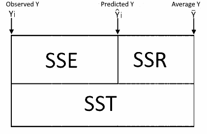
The least squares method is used to calculate the coefficients b and a. This approach chooses the line that will minimize the sum of the square length of the real values (Y) from the linear line (ŷ).
$$Min(\sum_{i=1 }^{n}(\hat y_i-y_i)^2)$$ $$b_1=\frac{\sum_{1}^{n}(x_i-\bar{x})(y_i-\bar{y}) }{\sum_{1}^{n}(x_i-\bar{x})^2}\\ b_0=\bar{y}-b_1\bar{x}$$ R² is the ratio of the variance explained by X with the total variance (Y)
R is the correlation between X and Y
$$R=a*\frac{var(x)}{var(y)}$$

Multiple Linear Regression (Go to the calculator)

When having more than one dependent variable, the multiple regression will compare the following hypothesis, using the F statistic:
H₀: Y = b₀
H₁: Y = b₀+b₁X₁+...+b_pX_p

Choosing the independent variables is an interactive process. You should check each coefficient for the following hypothesis:
H₀: b_i = 0
H₁: b_i ≠ 0

Each time you should remove only the one most insignificant variable (p-value > α) changing the "include" sign from √ to χ
After removing one insignificant variable, other insignificant variables may become significant in the new model.

Assumptions

• Linearity - a linear relationship between the dependent variable, Y and the independent variables, X_i
• Residual normality - the tool will run the Shapiro-Wilk test per each variable, but for the regression model, the only required normality assumption is for the residuals.
• Homoscedasticity, homogeneity of variance - the variance of the residuals is constant and does not depend on the independent variables X_i
• Variables - The dependent variable, Y, should be continuous variable while the independent variables, X_i, should be continuous variables or ordinal variables (ordinal example: low, medium, high)
• No Perfect Correlation (Multicollinearity) - between two or more independent variables, X_i.
• Independent observations

Overfitting

It is tempting to increase the number of independent variables to increase the model fitting, but you should beware that any additional independent variable may increase the fitting of the current data but will not improve the prediction of future data.

Cannot calculate the model

The tool will not be able to calculate the model when having one of the following problems. Technically it would not be able to calculate the inverse of the following matrix multiplication: X^tX

• Too many independent variables (Xi) or too small sample size.
  Solution: Reduce the number of independent variables or increase the sample size.
• Multicollinearity, two independent variables (Xi) has a perfect correlation (1).
  Solution: Remove one of the variables.

White test

Test for homoscedasticity, homogeneity of variance using the following hypothesis
$$ H_0: \hat\varepsilon_i^2=b_0\\ H_1: \hat\varepsilon_i^2=b_0+b_1\hat Y_i+b_2\hat Y_i^2 $$ While the ε is the residual and Ŷ is the predicated Y, the test will run a second regression with the following variables:
Independent variable: Y' = ε².
Dependent variables: X'₁=Ŷ, X'₂=Ŷ ².

The tool uses the F statistic which is the result of the second regression. Another option is to use the following statistic: χ²=nR'² while n is the sample size and R'² is the result of the second regression.

The regression is robust for the homoscedasticity assumption violation. If you do not meet this assumption, please try one of the following:

• Try to transform the dependent variables X_i, square root for count variable, log for skew variable and other
• You may be missing an independent variable or combination (x_i or x_ix_j or x_i²)
• Weighted regression

Regression calculation

Calculate the regression's parameters without matrices is very complex, but it is very easy with the matrix calculation.
p - number of independent variables.
n - sample size.

Y - dependent variable vector (n x 1). $$\hat Y (predicted \space Y) \space vector (n x 1).$$ X - independent matrix (n x p+1). Ε - Residuals vector (n x 1). B - Coefficient vector (p+1 x 1) $$Y=\begin{bmatrix} &Y_1\\ &Y_2\\ & :\\ &Y_n \end{bmatrix} \hat Y=\begin{bmatrix} & \hat Y_1\\ & \hat Y_2\\ & :\\ & \hat Y_n \end{bmatrix} X=\begin{bmatrix} &1 &X_{11} &X_{12} & .. &X_{1p} \\ &1 &X_{21} &X_{22} & .. &X_{2p} \\ & : & : & : & : & : \\ &1 &X_{n1} &X_{n2} & .. &X_{np} \end{bmatrix}\\ Ε=\begin{bmatrix} & \varepsilon_1\\ & \varepsilon_2\\ & :\\ & \varepsilon_n \end{bmatrix} B=\begin{bmatrix} &b_0\\ &b_1\\ &b_2\\ & :\\ &b_p \end{bmatrix}\\$$ Y = XB + Ε, is equivalent to the following equation: Y = b₀ + b₁X₁ + b₂X₂+...+b_pX_p+ε
$$ B = (X'X)^{-1}X'Y\\ \hat Y=XB\\ Ε=Y-\hat Y$$ Calculate the Sum of Squares, Degrees of Freedom and the Mean Squares

$$Total: \space SST=\sum_{1}^{n}(Y_i-\bar{Y})^2, \quad DFT=n-1\\ Regression: \space SSR=\sum_{1}^{n}(\hat{Y}_i-\bar{Y})^2, \quad SSR=SST-SSE, \quad DFR=p, \quad MSR=\frac{SSR}{DFR}\\ Residual: \space SSE=\sum_{1}^{n}(Y_i-\hat{Y})^2, \quad SSE=Ε'Ε, \quad DFE=n-p-1, \quad MSE=\frac{SSE}{DFE} \\ Variance(\hat{Y})=\frac{\sum_{1}^{n}(\hat{Y}_i-\bar{Y})^2}{n}\\ Variance(Y)=\frac{\sum_{1}^{n}(Y_i-\bar{Y})^2}{n}\\ R \space Squared: \space R^2=\frac{Explained\: variance}{Total\: variance}=\frac{Variance(\hat{Y})}{Variance(Y)} =\frac{SSR}{SST}=1-\frac{SSE}{SST}\\ Regression statistic: \space F=\frac{MSR}{MSE} \quad(DFR,DFE)\\ \space\\ Covariance(B)=MSE(X'X)^{-1}\\ Var(B)=diagonal(Covariance(B))$$ The standard error (SE) vector is the standard deviation of B vector. $$SE(B)=Sqrt(Var(B))$$ Following T vector that contains the t statistics for each coefficient significance $$T_i=\frac{B_i}{SE_i}(DFE)$$ DFT - Since you know the average, if you know (n-1) values of y, you can calculate the missing y_i based on Y
Coefficients Confident Interval $$Lower=B_i+SE_i+t_{\alpha/2}(DFE)\\ Upper=B_i+SE_i+t_{1-\alpha/2}(DFE)\\ $$

Regression model without an intercept (without constant)

You use this model when you are sure that the line must go through the origin.
Usually it is not recommended to use the model without the intercept! especially when the data used doesn't include values near the origin, in this case the model may be linear around the observations, but not linear near the origin

The calculation is similar to the model with the intercept except for the following:
The X Matrix doesn't include the first column of 1.
$$ X=\begin{bmatrix} &X_{11} &X_{12} & .. &X_{1p} \\ &X_{21} &X_{22} & .. &X_{2p} \\ & : & : & : & : \\ &X_{n1} &X_{n2} & .. &X_{np} \end{bmatrix}\\ B=\begin{bmatrix} &b_1\\ &b_2\\ & :\\ &b_p \end{bmatrix}\\$$ Y = XB + Ε, is equivalent to the following equation: Y = b₁X₁ + b₂X₂+...+b_pX_p+ε

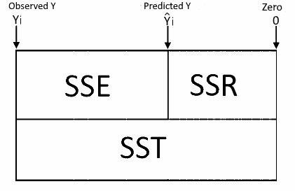
In the model without the intercept, the SST and the SSR are related to zero instead of Y average (y̅). Therefore you can't compare the R-squared of the model with the constant to the R-squared of the model without the constant. Since the SST calculation isn't related to the average, there is no need to reduce one degree of freedom. So DFT = n.
Hence DFE = DFT - DFR = n - p.
$$ Total: \space SST=\sum_{1}^{n}(Y_i-0)^2, \quad DFT=n\\ Regression: \space SSR=\sum_{1}^{n}(\hat{Y}_i-0)^2, \quad SSR=SST-SSE, \quad DFR=p, \quad MSR=\frac{SSR}{DFR}\\ Residual: \space SSE=\sum_{1}^{n}(Y_i-\hat{Y})^2, \quad SSE=Ε'Ε, \quad DFE=n-p, \quad MSE=\frac{SSE}{DFE} \\ $$ H₁: Y = b₁X

Numeric Example

Following the data as a matrix structure.