Proportion Test

One sample proportion test calculator Two sample proportion test calculator

The proportion test compares the sample's proportion to the population's proportion or compares the sample's proportion to the proportion of another sample.

One sample proportion test (Go to the calculator)

We use this test to check if the known proportion is statistically correct, based on the sample proportion and the sample size.
the null hypothesis assumes that the known proportion is correct. The statistical decision will be based on the difference between the know proportion and the sample proportion.

You may choose between the binomial test, which is more accurate, especially for the small sample size and the normal approximation.
We recommend using only the binomial test. If the tool won't be able to calculate the binomial distribution it will automatically calculate base on the normal approximation. depend on the sample size and how close is x to np. for a sample size smaller than 1000 any combination will be calculate based on the binomial distribution (when choosing the binomial test).

Example: It is known that the proportion of newborn males in the human race is 0.5122. The residence of Brobdingnag claims that in their country the proportion is smaller.

Assumptions

Binomial distribution - the probability for an event is identical
The population's proportion, p₀, is known.

Required sample data

Calculated based on a random sample from the entire population.

p̂ - Sample proportion or x number of successes.
If you enter a value between 0 and 1 the tool will assume you entered p̂ , if you fill number bigger than 1, the tool will assume you entered the number of successes x.
n - Sample size

Test statistic

Normal approximation
x distribution is binomial.
The binomial mean is μ = np, and the binomial standard deviation is: $$\sigma_x=\sqrt{np(1-p)}$$ The proportion p distributes with a mean of p₀ and the following standard deviation: $$\sigma_p=\sqrt{\frac{p_0(1-p_0)}{n}}$$ Following the normal statistic: $$z=\frac{(\hat{p}-p_0)+c}{\sqrt{\frac{p_0(1-p_0)}{n}}}$$ Since the normal distribution is continuous and the binomial distribution is discrete we may use the continuous correction to improve a bit the result.
$$ p>p_0:\qquad\quad c=-\frac{1}{2n}\\ p\lt p_0:\qquad\quad c=-\frac{1}{2n}\\ |p-p_0|\lt \frac{1}{2n}:\;c=0 $$ Exact test - binomial distribution
When using the binomial distribution the test statistic is the number of successes: X.

Since the distribution is discrete there is a big difference between lower/greater or lower equal/greater equal (unlike continuous distribution). It is also more complicated to calculate the 2 tailed p-value as the distribution is not symmetrical, and you can't get the exact the same value in the opposite tail.
The following will use the example of n = 8 and p = 0.25

x	p(X=x)	p(X≤x)	p(X≥x)
0	0.100112915	0.100112915	1
1	0.266967773	0.367080688	0.899887085
2	0.311462402	0.678543091	0.632919312
3	0.207641602	0.886184692	0.321456909
4	0.086517334	0.972702026	0.113815308
5	0.023071289	0.995773315	0.027297974
6	0.003845215	0.99961853	0.004226685
7	0.000366211	0.999984741	0.00038147
8	1.52588E-05	1	1.52588E-05

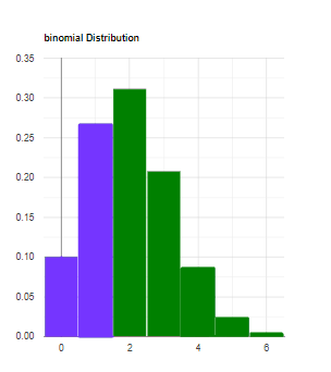
When x = np, x equals exactly the mean, x located in the middle of the distribution and p-value equals 1.
Left-tailed

$$p-value=p(X\le x)=\sum_{i=0}^{x}\binom{n}{x}p^xq^{n-x}$$ Example: x=1.
Since x < np, x located on the left side of the distribution. (1<8*0.25)
p-value=p(X≤1)=0.367081.

Right-tailed

$$p-value=p(X\ge x)=\sum_{i=x}^{n}\binom{n}{x}p^xq^{n-x}$$ Example: x=4.
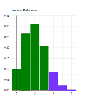
Since x > np, x located in the right side of the distribution. (4>8*0.25)
p-value=p(X ≥ 4)=1-p(X ≤ (4-1))=0.113815.

Two-tailed

Find the tail in one size based on x.
Find the x' on the opposite tail, with the greater density that is less or equal to the density of x.
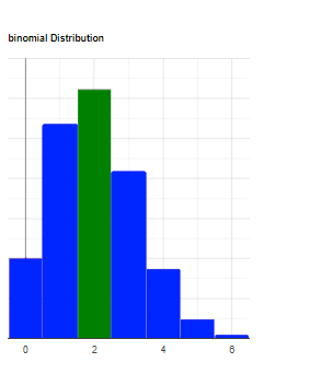
For example, if x on the left tail: $$p-value=p(X\le x) + p(X\ge x')\\ p-value=\sum_{i=0}^{x}\binom{n}{x}p^xq^{n-x} + \sum_{i=x}^{n}\binom{n}{x}p^xq^{n-x}$$ Example: x=1.
On the left side: p(X=1)=0.266968
On the right side: p(X=3)=0.207642. p(x=2)=0.311462, so x'=3.
p-value = p(X≤1) + p(X ≥ 3) = 0.367081 + 0.321457 = 0.6885376.

Effect size

The tool calculates the h effect size.
$$\varphi(p)=2arcsine(\sqrt{p})\\ h=\varphi(p̂)-\varphi(P_0)$$ Cohen's interpretation for the h effect size:
Small effect - 0.2.
Medium effect - 0.5.
Large effect - 0.8.

Two Sample proportion test (Go to the calculator)

We use this test to check if the proportion of group1 is the same as the proportion of group2.
The tool's null hypothesis assumes that the known difference between the groups is zero (using only the pooled variance).
Example: compares the proportion of good oranges between two fields, base on a sample from each group. H₀ assumes the proportions are identical.

Assumptions

Binomial distribution - the probability for an event within each group is identical

Required sample data

Calculated based on a random sample from the entire population

p̂₁, p̂₂ - Sample proportions or x₁,x₂ number of successes.
If you enter a value between 0 and 1 the tool will assume you entered p̂ , if you fill number bigger than 1, the tool will assume you entered the number of successes x.
n₁, n₂ - Sample sizes

Test statistic

Normal approximation
X₁ and X₂ distributions are binomial.
The difference between P₁ and P₂ assumes to distributes with mean equals 0, and Following the normal statistic: $$z=\frac{(\hat{p_1}-\hat{p_2})-0}{\sigma}\\$$ There are two ways to calculates the standard deviation σ based on the null assumption.

Pooled variance
When H₀ assumes p₁ - p₂ = 0, since the standard deviation of the binomial distribution is based on p, this assumption also includes the assumption that the standard deviation is identical for the two samples, hence we should calculate the pooled variance. based on the two samples together. $$ \hat{p}=\frac{x_1+x_2}{n_1+n_2}=\frac{n_1\hat{p}_1+n_2\hat{p}_2}{n_1+n_2}\\ Var_{pooled}=Var_1+Var_2\\ Var_{pooled}=\frac{p_1(1-p_1)}{n_1}+\frac{p_2(1-p_2)}{n_2}\\ $$ Since we assume that p₁=p₂: $$ \hat{p_1}=\hat{p_2}=\hat{p}\\ Var_{pooled}=\frac{\hat{p}(1-\hat{p})}{n_1}+\frac{\hat{p}(1-\hat{p})}{n_2}\\ \sigma_{pooled}=\sqrt{\hat{p}(1-\hat{p})(\frac{1}{n_1}+\frac{1}{n_2})}\\ z_{pooled}=\frac{(\hat{p_1}-\hat{p_2})+c}{\sqrt{\hat{p}(1-\hat{p})(\frac{1}{n_1}+\frac{1}{n_2})}}\\ $$ Unpooled variance
The tool doesn't calculate the unpooled variance.
When H₀ assumes p₁ - p₂ = d, since the standard deviation of the binomial distribution is based on p, this assumption also includes the assumption that the standard deviation is not identical for the two samples, so we need to calculate the accumulate variance of two independent random variables: $$ Var_{unpooled}=Var_1+Var_2\\ \sigma_{unpooled}=\sqrt{\frac{\hat{p_1}(1-\hat{p_1})}{n_1}+\frac{\hat{p_2}(1-\hat{p_2})}{n_2}}\\ z_{unpooled}=\frac{(\hat{p_1}-\hat{p_2})+c}{\sqrt{\frac{\hat{p_1}(1-\hat{p_1})}{n_1}+\frac{\hat{p_2}(1-\hat{p_2})}{n_2}}}\\ $$ Since the normal distribution is continuous and the binomial distribution is discrete we may use the continuous correction to improve a bit the result.
$$ Right-tailed\;or\;Two\;tailed:\; c=\frac{1}{2n_1}+\frac{1}{2n_2}\\ Left-tailed\;or\;Two\;tailed:\; c=-\frac{1}{2n_1}+\frac{1}{2n_2}\\ $$

Effect size

The tool calculates the h effect size.
$$\varphi(p)=2arcsine(\sqrt{p})\\ h=\varphi(p̂_1)-\varphi(p̂_2)$$ Cohen's interpretation for the h effect size:
Small effect - 0.2.
Medium effect - 0.5.
Large effect - 0.8.