Power analysis

Statistical Power

The statistical power is the probability that a test will reject an incorrect H₀ for defined effect size. Researchers usually use a priori power of 0.8.

The statistical power complements the p-value to provide an accurate test result. While the p-value represents the probability of rejecting a correct H₀, an accepted H₀ does not guarantee that H₀ is correct. It only indicates that the probability of rejecting a correct H₀ (p-value), will be greater than the significant level(α), this risk that statisticians are not willing to take. Usually, α is 0.05, meaning there is a 5% chance of a type I error.

The smaller the power value is, the likelier it is that an incorrect H₀ will be rejected.

The statistical power depends on the statistic value of H₁. However, this H₁ statistic is not always defined. For example, there is no specific value for μ in H₁: μ != μ₀. Instead, an expected effect for the test to identify must be defined, to construct a particular distribution for H₁. This distribution is then compared with the H₀ distribution to calculate the power value.

There are a few factors which contribute to the power of a test:
The effect size ⇑ - the greater the effect size is, the stronger the test power due to the difficulty of distinguishing between an incorrect H₀ and a result obtained by chance.
The sample size ⇑ - the greater the sample size the stronger the test power, as the large sample size ensures a small standard deviation and more accurate statistics.
The significance level ⇓ - a lesser significance level accepts a bigger range for H₀ and therefore limits the ability to reject H₀, thereby lowering the power of the test.
The standard deviation ⇓ - the greater the standard deviation the weaker the test power.

You should determine the effect size and the significant level before you calculate the test power. The correct ways to increase the test power are to increase the sample size or to reduce the standard deviation (better process, more accurate measurement tool, etc)

Statistical power can be conducted on two different occasions:

A priori power

A priori test power is conducted before the study based on the required effect size. This method is recommended in order to ensure more effective and organized testing.
This tool calculates only the a priori power.

Observed power (post-hoc power)

The observed power is calculated after collecting the data, based on the observed effect.
It is directly correlated to the p-value. Generally, H₀ will be accepted when the observed effect size is small and therefore results in a weak observed power. On the contrary, when H₀ is rejected for this test, the observed effect will be large and the observed power will be strong.

Effect size

A measurement of the size of a statistical phenomenon, for example, a mean difference, correlation, etc. there are different ways to measure the effect size.

Effect size (unstandardized)

the pure effect as it, for example, if you need to identify a change of 1 mm in the size of a mechanical part, the effect size is 1mm

Standardized effect size

Used when there is no clear cut definition regard the required effect, or the scale is arbitrary, or to compare between different researches with different scales
this site uses the Cohen's d as Standardizes effect size

Expected Cohen's d $$ d=\frac{\mu_1-\mu_0}{\sigma_{population}}$$ Observed Cohen's d $$ d=\frac{\overline{x}-\mu_0}{\sigma_{population}} $$ Cohen's standardized effect is also named as following:

• 0.2 - small effect.
• 0.5 - medium effect.
• 0.8 - large effect.

Chi Squared effect size

Following the Cohen's w: $$ w=\sqrt{\sum_{i=1}^{n}\frac{(p_{0i}-p_{1i})^2}{p_{0i}}} $$

Effect ratio

Used when there is no clear cut definition regard the required effect, and compare the effect size to the current expected value.
Calculate the effect size as a ratio of the expected value

Power calculation

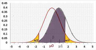
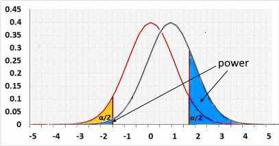
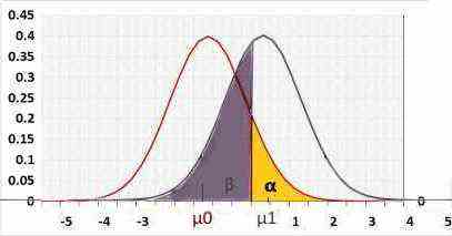
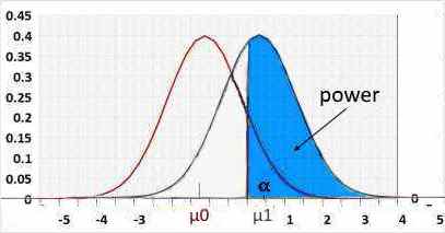
Statistical power = 1 - β .

β - the probability of a type II error, meaning the test won't reject an incorrect H₀.
R₁ - left critical value.
R₂ - right critical value.

Choose β or power in the following charts

Two-tailed

Rejected H₀ when: statistic < R1 or statistic > R2

Left tail

Rejected H₀ when statistic < R1.
H₁ assumes the statistic is "lesser than" while H₀ assumes "greater than". Hence the change/effect size should be negative.
Using a positive change will result in a small power because the statistic is actually "greater than", and supports H₀, not H₁.

β - type II error
Power

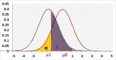
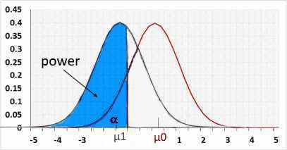
Right tail

Rejected H₀ when statistic>R2.
H₁ assumes the statistic is "greater than" while H₀ assumes "lesser than". Hence the change/effect size should be positive.
Using a negative change will result in a small power because the statistic is actually "lesser than", and supports H₀, not H₁.

β - type II error
Power

One sample z-test power

Expected Cohen's d: $$ d=\frac{\mu-\mu_0}{\sigma_{population}}=\frac{change}{\sigma_{population}} \\ statistic=\frac{\bar x-\mu_0}{\sigma_{statistic}} \\ H_0: \bar x \sim N(\mu_0 , \sigma_{statistic}) \\ H_1: \bar x \sim N(\mu_0 + change , \sigma_{statistic}) \\ \sigma_{statistic}={\frac{\sigma_{population}}{\sqrt{n} }} \\ $$

Two tailed

Assuming μ₁ > μ₀ assuming the opposite will have the same result. $$ \mu>\mu_0 \;\rightarrow change=\mu-\mu_0\\ R_1=\mu_0+Z_{\alpha/2}\,\sigma_{statistic} \\ R_2=\mu_0+Z_{1-\alpha/2}\,\sigma_{statistic} \\ \beta=p(R_1 < statistic < R_2\,|\,H1) \\ =p(statistic < R_2)-p(statistic < R_1) \\ =p(Z < \frac{R_2-\mu_0 -change}{\sigma_{statistic}})-p(Z < \frac{R_1-\mu_0-change}{\sigma_{statistic}}) \\ =p(Z < \frac{\mu_0+Z_{1-\alpha/2}\;\sigma_{statistic}-\mu_0 -change}{\sigma_{statistic}})-p(Z < \frac{\mu_0+Z_{\alpha/2}\;\sigma_{statistic}-\mu_0-change}{\sigma_{statistic}}) \\ =p(Z < Z_{1-\alpha/2}-\frac{change}{\frac{\sigma_{population}}{\sqrt{n} }})-p(Z < Z_{\alpha/2}\ - \frac{change}{\frac{\sigma_{population}}{\sqrt{n} }}) \\ \beta= p(Z < Z_{1-\alpha/2} - d\sqrt{n}) - p(Z < Z_{\alpha/2} - d\sqrt{ n}) \\ \bf power=1-p(Z < Z_{1-\alpha/2} - d\sqrt{ n}) + p(Z < Z_{\alpha/2} - d\sqrt{ n }) $$

Right tail

$$ \mu>\mu_0 \;\rightarrow change=\mu-\mu_0\\ R_2=\mu_0+Z_{1-\alpha}\,\sigma_{statistic} \\ \beta=p(statistic < R_2\,|\,H1) \\ =p(Z < \frac{R_2-\mu_0 -change}{\sigma_{statistic}}) \\ =p(Z < \frac{\mu_0+Z_{1-\alpha}\,\sigma_{statistic}-\mu_0 -change}{\sigma_{statistic}}) \\ =p(Z < Z_{1-\alpha}-\frac{change}{\frac{\sigma_{population}}{\sqrt{n} }}) \\ \beta= p(Z < Z_{1-\alpha} - d\sqrt{n})\\ \bf power=1-p(Z < Z_{1-\alpha} - d\sqrt{ n}) $$

Left tail

The same as right tail.

Two sample z-test power

Change - the change between the groups we expect the test to identify, reject the H₀ if the difference between the groups is equals or greater than change.
Expected Cohen's d: $$ d=\frac{\mu_2-\mu_1}{\sigma_{pool}}=\frac{change}{\sigma_{pool}} \\ \sigma_{pool}=\frac{\sigma1+\sigma2}{2}\\ H_0: (\bar x_2-\bar x_1) \sim N(0 , \sigma_{statistic}) \\ H_1: (\bar x_2-\bar x_1) \sim N(change , \sigma_{statistic}) \\ \sigma_{statistic}=\sqrt{ {\frac{\sigma_1^2}{n_1}+\frac{\sigma_2^2}{n_2}} } \\ $$ Lets define n_pool as: $$ n_{pool}=\frac{ n_1n_2(\sigma1^2+\sigma_ 2^2) }{ 2(n_2\sigma_1^2+n_1\sigma_2^2) }\\ $$ In the following calculation I chose μ₂ to be the value toward the tail in the one tail calculation, and toward the right tail in the two tailed calculation
An opposite assumption will have the same result.

Two tailed

The calculation is based on the following assumption, but the opposite assumption will have the same final result.
$$ \mu_2 > \mu_1 \;\rightarrow change=\mu_2-\mu_1\\ R_1=0+Z_{\alpha/2}\,\sigma_{statistic} \\ R_2=0+Z_{1-\alpha/2}\,\sigma_{statistic} \\ \beta=p(R_1 < statistic < R_2\,|\,H1) \\ =p(statistic < R_2)-p(statistic < R_1) \\ =p(Z < \frac{R_2-change}{\sigma_{statistic}})-p(Z < \frac{R_1-change}{\sigma_{statistic}}) \\ =p(Z < \frac{Z_{1-\alpha/2}\,\sigma_{statistic}-change}{\sigma_{statistic}})-p(Z < \frac{Z_{\alpha/2}\,\sigma_{statistic}-change}{\sigma_{statistic}}) \\ \beta=p(Z < Z_{1-\alpha/2}-\frac{change}{\sigma_{statistic}})-p(Z < Z_{\alpha/2}-\frac{change}{\sigma_{statistic}}) \\ or \: \beta= p(Z < Z_{1-\alpha/2} - d\sqrt{ n_{pool}}) - p(Z < Z_{\alpha/2} - d\sqrt{ n_{pool} }) \\ \bf power=1-p(Z < Z_{1-\alpha/2} - d\sqrt{ n_{pool}}) + p(Z < Z_{\alpha/2} - d\sqrt{ n_{pool} }) $$

Right tail

$$ \mu_2 > \mu_1 \;\rightarrow change=\mu_2-\mu_1\\ R_2=0+Z_{1-\alpha}\,\sigma_{statistic} \\ \beta=P(statistic < R_2 | H_1) = p(Z < \frac{R_2-change}{\sigma_{statistic}}) =p(Z < \frac{Z_{1-\alpha}\sigma_{statistic}-change}{\sigma_{statistic}} ) \\ \beta=p(Z < Z_{1-\alpha} - \frac{change}{\sigma_{statistic}}) \;or\; \beta =p(Z < Z_{1-\alpha} - d\sqrt{ n_{pool} })\\ $$ When calculate the sample size we can define n₁=n₂. $$\beta=p(Z < Z_{1-\alpha} - d\sqrt{n_1}) \\ \bf power=1-p(Z < Z_{1-\alpha} - d\sqrt{n_1}) \\ $$

Left tail

The result will be identical to the right tail. $$ \mu_2 < \mu_1 \;\rightarrow change=\mu_1-\mu_2\\ R_1=0+Z_{\alpha}\,\sigma_{statistic} \\ power=p( statistic < R_1) = p(Z < \frac{R_1-change}{\sigma_{statistic}}) \\ =p(Z < \frac{Z_{\alpha}\sigma_{statistic}-change}{\sigma_{statistic}} ) \\ power=p(Z < Z_{\alpha}- \frac{change}{\sigma_{statistic}} ) \\ \bf power=p(Z < Z_{\alpha} + d\sqrt{n_1}) $$ It is the same result as the right tail: $$ power= p(Z < -Z_{1-\alpha} + d\sqrt{n_1})=p(Z < -(Z_{1-\alpha} - d\sqrt{n_1}) )\\ = p(Z > Z_{1-\alpha} - d\sqrt{n_1}) \bf=1 - p(Z < Z_{1-\alpha} - d\sqrt{n_1} ) $$

T-test power

t distribution - When H₀ assumes to be correct the t statistic distribute t.
noncentral-t distribution (NCT) - When H₁ assumes to be correct the t statistic distribute noncentral-t.
$$ H_0: (statistic) \sim \color{blue}{t\,}(df) \\ H_1: (statistic) \sim \color{blue}{noncentral t}(df , noncentrality) \\ $$

One Sample or Paired-t
The paired t-test, after calculating the differences between the two groups, behave exactly as one sample t-test over the differences.

Change=μ-μ₀

Expected Cohen's d: $$d=\frac{\mu-\mu_0}{S}=\frac{change}{S} \\ statistic=\frac{\bar x-\mu_0}{S_{statistic}} \\ S_{statistic}=\frac{S}{\sqrt{n} } $$ n - sample size
S - the sample standard deviation of the population
df = n - 1
$$noncentrality=\frac{change}{S_{statistic}}=\frac{change}{\frac{S}{\sqrt{n}}}=d\sqrt{n}$$ Two Sample
Change=μ₂-μ₁
$$ d=\frac{\mu_2-\mu_1}{s_{population}}=\frac{change}{s_{population}} \\ S_{statistic}=\sqrt{\frac{(n_1-1)s_1^2+(n_2-1)s_2^2}{n_1+n_2-2}} \\ $$ S - the sample standard deviation of the population
$$ df = n_1+n_2-2 \\ noncentrality=\frac{change}{S_{statistic}}=\frac{change}{ S \sqrt{ \frac{1}{n_1}+\frac{1}{n_2} } }=d\sqrt{n}\\ $$ Lets define n as: $$ n=\frac{1}{\frac{1}{n_1}+\frac{1}{n_2}}\\ $$

Two tailed

Since it is two tail, choosing positive change or negative change will support identical result.
For this calculation I chose a positive change (change > 0)
$$ R_1=\mu_0+T_{\alpha/2} \, \sigma_{statistic} \\ R_2=\mu_0+T_{1-\alpha/2} \,\sigma_{statistic} \\ \beta=p(R_1 < statistic < R_2 \, | \, H1) \\ =p(statistic < R_2) - p(statistic < R_1) \\ =F_{df , d\sqrt{n} }(R_2) - F_{df,d\sqrt{n}}(R_1) \\ =F_{df , d\sqrt{n} }(R_2) - F_{df,d\sqrt{n}}(\mu_0+T_{\alpha/2} \, \sigma_{statistic}) \\ $$ $$ \beta= p(T < T_{1-\alpha/2} - d\sqrt{n}) - p(T < T_{\alpha/2} - d\sqrt{ n}) \\ \bf power=1-p(T < T_{1-\alpha/2} - d\sqrt{ n}) + p(T < T_{\alpha/2} - d\sqrt{ n }) $$

Right tail

H₁ assumes μ > μ₀ => change > 0
$$ R_2=\mu_0+T_{1-\alpha}\,\sigma_{statistic} \\ \beta=p(statistic < R_2\,|\,H1) \\ =p(Z < \frac{R_2-\mu_0 -change}{\sigma_{statistic}}) \\ =p(Z < \frac{\mu_0+Z_{1-\alpha}\;\sigma_{statistic}-\mu_0 -change}{\sigma_{statistic}}) \\ =p(Z < Z_{1-\alpha}-\frac{change}{\frac{\sigma_{population}}{\sqrt{n} }}) \\ \beta= p(T < T_{1-\alpha} - d\sqrt{n}) \\ \bf power=1-p(T < T_{1-\alpha} - d\sqrt{ n}) $$

Left tail

The same as right tail.

Chi-squared test power

Chi-squared distribution - When H₀ assumes to be correct the test statistic distribute chi-squared.
Noncentral-chi-squared distribution - When H₁ assumes to be correct the test statistic distribute noncentral chi-squared .
$$ H_0: (statistic) \sim \color{blue}{\chi^2\,}(df) \\ H_1: (statistic) \sim \color{blue}{noncentral\ \chi^2}(df, noncentrality) \\ $$

Right tail

H₁ assumes change > 0
w - required effect size.
$$ R_2=\chi^2_{1-\alpha}(df) \\ noncentrality=nw^2\\ \beta=p(statistic < R_2\,|\,H1) \\ \beta=noncentral \chi^2(R_2,df,nw^2)\\ \bf power=1-noncentral\ \chi^2(R_2,df,nw^2)\\ $$